
Reviewed captions define residuals as observed minus predicted and connect their signs to positions relative to a fitted line.
A model prediction is not an observation
Suppose a school workshop uses a fitted rule to predict how many minutes an assembly takes: predicted time equals 5 plus 3 times the number of components. The input is a component count, and the output is time in minutes. An actual assembly can finish above or below the predicted time. Keeping those two quantities separate is the first step in evaluating the rule.
The linked Khan Academy video introduces a residual through a bicycle-fitting example. Its reviewed captions define the difference between an observed output and a model prediction, then interpret the sign. We read the full available instructional caption range from 0 to 291 seconds. The workshop data, diagrams, model comparisons and exercises below are newly authored. The article uses the source method without copying its bicycle example.
Read one vertical difference
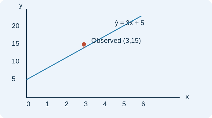
For an assembly with three components, our rule predicts 5+3(3)=14 minutes. Suppose the observed time is 15 minutes. Its residual is 15−14=1 minute. The marked observation lies one output unit above the line at the same input. Use a vertical comparison: moving horizontally would compare component counts, which are different units and answer a different question.
In the original graph, the observed point (3,15) and predicted point (3,14) share the same horizontal position because they refer to the same three-component assembly. Their vertical separation is one minute. Read the labeled axes before comparing the two outputs, and keep the residual in the output unit. A vertical difference in minutes cannot be replaced by a horizontal difference in component counts.
Let the sign describe the miss
Consider a second assembly with four components and an observed time of 15 minutes. The rule predicts 17 minutes, so the residual is −2 minutes. The negative sign tells us that the observation lies below the predicted output. It also means that the model overpredicted the time by two minutes. Saying merely that the error is two loses the direction of that disagreement.
A third assembly has five components and an observed time of 20 minutes. The prediction is also 20, so its residual is zero. That one exact agreement does not establish that the model is perfect. A model should be evaluated over a relevant set of observations. An observation on the line is evidence about that observation, while a general claim requires a broader comparison and an appropriate collection process.
Compare models on the same observations
For the three original assemblies, the residual list is [1, −2, 0]. The sum of squared residuals is 1+4+0=5 square minutes. Squaring each residual before adding prevents a positive miss and a negative miss from canceling. If you instead add the signed residuals first and then square, you obtain 1, which is a different quantity and cannot be substituted for the stated loss.
Now compare a candidate rule that raises the intercept from 5 to 6 while keeping slope 3. Its predictions are [15, 18, 21], so the residuals become [0, −3, −1]. Their squared sum is 10. On these same three observations, the original rule has the smaller squared-error total. This is our instructional model-comparison extension. We have not proved that either candidate is the least-squares fit among all possible lines.
Separate computation from inference
A smaller squared-error total does not establish a causal relationship. The number of components might be related to assembly time, but operator experience, tools or material differences could also matter. A fitted rule summarizes a relationship under its observed conditions. It does not by itself tell us what would happen after an intervention or whether the pattern extends far beyond the measured inputs.
Predictions inside the observed input range are interpolations; predictions well outside it are extrapolations. Our three assemblies have inputs 3, 4 and 5. Predicting for 4 is within that range, while predicting for 40 would require a strong assumption that the same rule continues to apply. The arithmetic 5+3(40)=125 is easy; the reasonableness of applying that rule at 40 is a separate modeling question.
Transfer the idea without memorizing a sign
Try a new case: predicted output is 2x+7, input x is 6, and the observed output is 16. First compute the prediction, 19. Next subtract predicted from observed: 16−19=−3. Explain the sign in words before checking a choice: the observation is three output units below the prediction, so the model overpredicts by three units. This explanation prevents the common reversal to positive three.
If only the intercept increases by 4, every prediction rises by 4 while the observations stay fixed. The new residual is therefore −7, not 1. This final change tests whether you understand what is held constant. In ACT bivariate-data questions, identify input, prediction, observation, residual and the requested comparison explicitly. Those labels keep a short calculation connected to the model it is meant to evaluate.
PAUSE & TRYPrediction is2x+7, input6 and observed output16. What is the residual?Reveal explanation
−3:16−(2×6+7)=16−19.
Turn the idea into practice.
A fresh set will help you use the relationship with different numbers.
Practice this skillEvidence & editorial note
Freshly acquired English captions. Original examples and diagrams; no transcript republication. Read 0–291 seconds; three-observation loss comparison and inference discussion are original extensions.
Brief source synopsis and independently authored instructional companion.
Caption track SHA-256: f9bdf2379c4d07701aa469b6df5f4976dfa2ce1e5a0fc839938238137851a886
Source segment references are retained in the catalog. Full captions remain in the local research archive.