
The reviewed opening captions distinguish mean, median, mode and range after sorting observations.
Decide what the summary must describe
A summary is useful only when it matches a question. Imagine a student volunteer records the number of books returned during five short intervals: 2, 3, 3, 4 and 13. The list has an unusually busy final interval. A question about the average workload, the middle interval or the most common count will not necessarily have the same answer. Before reaching for a formula, identify the meaning of the requested statistic.
The reviewed opening caption segment of the linked video sorts observations and distinguishes mean, median, mode and range. These general methods support ACT statistics foundations. The book-return example, interpretations and comparisons below are newly authored. We reviewed the captions from 2 to 180 seconds; this is a focused companion to those concepts, not a transcription or a review of the entire source video.
Use a frequency table without losing observations
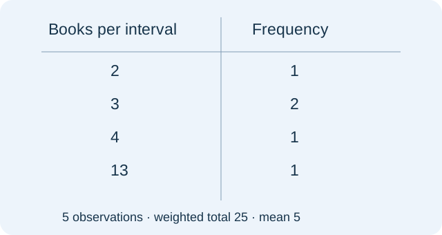
The original diagram records the same five observations in a frequency table. A count of 2 occurs once, 3 occurs twice, 4 occurs once and 13 occurs once. The frequencies total five; the weighted total is 2 times 1 plus 3 times 2 plus 4 times 1 plus 13 times 1, which equals 25. Therefore the mean is 25 divided by 5, or 5 books per interval.
A common error averages the four distinct values and obtains 5.5. That procedure gives every distinct value equal weight and discards the fact that 3 appeared twice. The table has four rows, but it describes five intervals. Write the number of observations separately from the number of categories before calculating. A frequency is a count of repeated observations, not a new observation to include in the value column.
Separate center from spread
The median is 3 because the sorted list has five positions and the third position is 3. The mode is also 3, because that count appears more frequently than any other. Their agreement is incidental: the definitions are different. For the list 2, 2, 5, 8, 9, the mode is 2 while the median is 5. This contrasting example checks whether you are using a definition rather than copying a familiar answer.
The range of the book-return counts is 13 minus 2, or 11. It describes the distance from the smallest to the largest observation, not where the data are centered. Reporting 13 gives the maximum instead of the range. Reporting 5 gives the mean instead of a spread measure. The units remain books per interval for this range because subtraction preserves the measurement unit.
Test the effect of an unusual observation
Now replace the busy interval of 13 books by an interval of 23 books, leaving the other four intervals unchanged. The new total is 35, so the mean becomes 7. The median stays 3, the mode stays 3 and the range becomes 21. The changed observation affects the total and the upper extreme, but it does not change which observation occupies the middle position.
This comparison explains why a median can better describe a typical interval when a distribution has an extreme tail, depending on the question being asked. It does not mean that the mean is wrong. If you need to schedule enough staff for the total workload, the total and mean may still matter. Avoid treating the choice of summary as a contest with one universally best measure.
PAUSE & TRYWhat happens to the median when 13 is replaced by 23?Reveal explanation
It remains 3: the sorted middle position is unchanged.
Combine groups by recovering their totals
Suppose one student works two shifts with a mean of 6 returned books, while another works three shifts with a mean of 11. The combined total is 2 times 6 plus 3 times 11, or 45. Across five shifts, the combined mean is 9. Averaging the two means gives 8.5 and assigns equal weight to groups that have different sizes.
This weighted example is our ACT teaching extension beyond the brief source synopsis. It connects group summaries to the same total-divided-by-count principle. When group sizes are equal, an ordinary average of group means works; unequal sizes require weights, even if special equal-mean cases happen to give the same result. Check that a combined mean falls between the group means when all weights are positive.
Make a small claim and check its limits
Five observed intervals describe those intervals. They do not automatically establish what happens in every library, at every hour or in every month. Generalizing requires a sampling design and a clearly defined population. These introductory calculations should therefore be accompanied by a plain statement of what was measured and how the measurements were collected.
For practice, add 4 to every original book-return count. The new mean is 9 and the new median is 7, while the range remains 11. Explain the unchanged range by subtracting the new extremes, 17 minus 6. Use that explanation to distinguish a shift in location from a change in spread. This article builds a focused statistics habit; independent educator review and full audiovisual review remain pending, and no ACT score is inferred from these exercises.
Turn the idea into practice.
A fresh set will help you use the relationship with different numbers.
Practice this skillEvidence & editorial note
Newly acquired caption evidence for a missing statistics topic. Only 2–180 seconds reviewed. All book-return examples and diagram are original. Weighted means and sampling comments are clearly original instructional extensions. Full audiovisual review pending.
Brief source synopsis plus original teaching extension.
Caption track SHA-256: a8ed7e4d9ff08b8af84d2a3915fd1d1c7c98829764bdc3a61a4a6e63c269f95b
Source segment references are retained in the catalog. Full captions remain in the local research archive.