
Khan Academy uses a bicycle-rental context to distinguish a recorded response from a fitted prediction. The source defines a residual as actual minus predicted, then interprets a negative residual as a point below the line. The chapters link those moments. This SAT companion uses a different original data set and adds its own checks about units, model comparison and the limits of association.
Give the two outputs different names
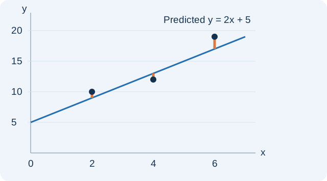
A model output and an observed output can refer to the same input without being equal. Write the model prediction as ŷ to keep it separate from the recorded value y. In the original example here, the supplied model is ŷ=2x+5. Our observations are (2,10), (4,12) and (6,19). We are evaluating this given model; we are not claiming it is a fitted least-squares line for these three observations.
At x=2, the prediction is nine but the observation is ten. At x=4, the prediction is thirteen but the observation is twelve. Those disagreements are information about the model’s errors, not reasons to replace an observed value with the model value. Keep the input and both outputs visible while calculating.
Read a residual as a vertical difference
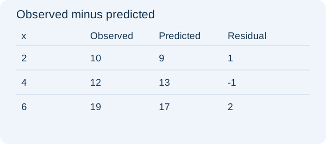
A residual is observed minus predicted at the same input. For the first point,10−9=1. For the second,12−13=−1. For the third,19−17=2. The orange segments in the diagram connect each observed point to the supplied line vertically. A positive residual places the observation above the line; a negative one places it below.
The sign is not a verdict that the observation is good or bad. It reports direction. A negative residual means that this model’s prediction exceeded the actual response. It is also not the shortest perpendicular distance to the line. Standard regression residuals compare y values while keeping x fixed, so a geometric distance measured in another direction answers a different question.
PAUSE & TRYAt x=4, does the supplied model overpredict or underpredict?Reveal explanation
It overpredicts by 1 output unit, because predicted 13 exceeds observed 12.
Use a table to audit the signs
The calculation table lists every input beside its observed value, prediction and residual. Recompute each prediction from the model rather than copying a neighboring observation. This matters when a table has many rows or the input values are not equally spaced. A residual is attached to a particular row, not to a gap between consecutive rows.
The residuals in this example sum to two. That is allowed because the supplied line was not asserted to be the least-squares fit with an intercept for these three points. Do not impose a property of a special fitted model on an arbitrary prediction rule. The task here is to interpret given information and retain the conditions under which a shortcut would apply.
Recover the hidden observation
Suppose a different record has x=5 and residual −3 under the same rule. Its prediction is 2(5)+5=15. Rearranging the definition gives observed=predicted +residual, so its observed value is twelve. Subtracting the residual would instead give eighteen and put the point on the wrong side of the line.
A practical check is to run the definition again:12−15=−3. This is stronger than checking only the sign, because it verifies the magnitude as well. If outputs measure liters, the observation, prediction and residual all measure liters. The slope would have output-units per input-unit; it should not be substituted for a residual.
PAUSE & TRYA prediction is 22 and its residual is +4. What was observed?Reveal explanation
26. The observation is four output units above the prediction.
Compare model patterns carefully
For equal input steps, outputs 3,6,12 have constant ratio two but unequal differences three and six. They support an exponential pattern over those points. Outputs 3,6,9 instead have constant difference three. This comparison helps choose a candidate model, but neither short table proves a unique underlying real-world law.
Residual patterns provide another diagnostic. A sequence of errors that rises consistently with input can suggest that a proposed line is missing part of the relationship. Three observations cannot settle every modeling question. Treat the pattern as a reason to investigate, rather than as proof of a particular replacement formula. Keep the prediction rule, observation range and units attached to the conclusion.
Distinguish prediction from a causal claim
A positive association between library visits and books borrowed may help describe the observed sample. It does not, by itself, isolate what would happen if an intervention changed a person’s visits. Other factors, such as reading habits or access, could influence both variables. An observational model and a randomized treatment comparison answer different questions.
Likewise, a small residual inside the observed input range does not validate a prediction far outside that range. Extrapolation assumes that the relationship continues. A model can fit existing observations well and still fail where capacity limits or a new process changes the behavior. State that boundary before treating a computed output as a practical forecast.
Finish with a three-part check
First, identify which output the prompt requests: observation, prediction or residual. Second, calculate using the input for that same record and keep the subtraction order explicit. Third, interpret the sign in words with the output unit. These checks address different mistakes and can be completed without drawing a detailed graph.
For a final transfer, use ŷ=3x+2 at x=4 with observed y=11. The prediction is fourteen and the residual is −3, so the model overpredicts by three output units. Compare that result with the source chapter’s interpretation of a point below a fitted line. Then practice the linked families, which separately ask for residuals, recovered observations, table patterns and appropriate observational claims.
PAUSE & TRYIf the observed value rose from 11 to 16 while the prediction stayed 14, what would the residual become?Reveal explanation
+2. The point would move from below the model to above it.
Turn the idea into practice.
A fresh set will help you use the relationship with different numbers.
Practice this skillEvidence & editorial note
All 109 normalized caption segments were read. The first spoken regression expression is corrupted by automatic captions, while later substitution gives clearer fractions; this article does not reproduce the source equation or data. Original data, plots and calculations below are Slope work. The video is labeled AP Statistics but the selected residual concept supports SAT bivariate-data foundations; regression derivation is outside this companion. Full audiovisual review remains pending.
Brief source synopsis; original teaching text, examples, and SVG diagrams.
Caption track SHA-256: f9bdf2379c4d07701aa469b6df5f4976dfa2ce1e5a0fc839938238137851a886
Source segment references are retained in the catalog. Full captions remain in the local research archive.