
The inspected captions explain class widths, frequency densities and histogram construction. Grouped summaries below are an original teaching extension, not a claim about additional video coverage.
A grouped picture preserves counts, not every value
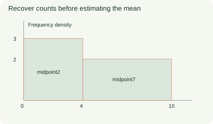
Suppose a histogram has a bar from 0 to 4 with density 3 and another from 4 to 10 with density 2. Their frequencies are 4×3=12 and 6×2=12, for a total of 24 observations. Those counts are recoverable exactly from the supplied grouped representation. The individual observations are not: the first 12 could be spread throughout their interval or clustered near one edge. This difference between known counts and unknown within-class locations explains why some summaries are exact and others must be estimates. The figure labels the boundaries and densities, keeping the available information separate from quantities calculated later.
Use midpoints to estimate a mean
The midpoint of the first class is 2 and the midpoint of the second is 7. Replacing every observation by its class midpoint gives an estimated total of 12×2+12×7=108, and an estimated mean 108/24=4.5. The weighted calculation matters even when the two class counts happen to be equal. In general, add midpoint times frequency for every class, then divide by the total frequency. Do not divide by the number of classes unless each class has equal frequency and you have explicitly reduced the weighted expression. The midpoint is a representative assumption, not a recovered individual measurement.
Change the frequencies to test the method
Consider a second original table with the same intervals but frequencies 8 and 16. The estimated total is 8×2+16×7=128 and the total frequency is 24, giving estimated mean 16/3, approximately 5.333. The simple average of the two midpoints is still 4.5, so it now disagrees with the correctly weighted estimate. The larger class count pulls the mean toward 7. This contrast is a quick way to test whether a method is using the actual frequencies or only the table’s rows. It also separates class width from frequency: width determines density, while frequency determines the weight in a grouped mean.
PAUSE & TRYFor midpoints 2,7 with frequencies 8,16, estimate the mean.Reveal explanation
(16+112)/24=16/3.
Build cumulative counts from the recovered frequencies
For the first histogram, cumulative frequency reaches 12 at boundary 4 and 24 at boundary 10. The total count up to a boundary includes every earlier class. To find the count between two boundaries, subtract the earlier cumulative total from the later one. For example, if a different table gives 18 observations at or below 10 and 46 at or below 20, then 28 lie above 10 and at or below 20. Adding those cumulative counts would count the earlier observations twice. A cumulative display changes the representation again, but it cannot restore individual values that were already lost when the data were grouped.
Interpret percentiles as estimates from grouped data
A sample of 80 has its upper quartile read at cumulative count 60 and lower quartile at cumulative count 20. The corresponding horizontal values must then be read from the cumulative curve. If those values are 30 minutes and 12 minutes, the interquartile range is 18 minutes. Subtracting the vertical counts 60−20 gives 40 observations, which has the wrong meaning and units for an interquartile range. A curve drawn through grouped cumulative data supports estimated positions within classes. Explain the interpolation assumption and avoid presenting the resulting quartiles with more precision than the supplied graph can justify.
PAUSE & TRYQuartiles read as 12 minutes and 30 minutes give which IQR?Reveal explanation
18minutes; subtract measurement values, not cumulative counts.
Distinguish a teaching extension from a video claim
The inspected source captions explain class width, frequency density and drawing histogram bars. The grouped-mean and cumulative-frequency work in this companion is an original extension from the recovered class counts; these additional topics are not claimed to have been taught in the selected source segment. This boundary matters because a source can support one prerequisite without supporting every later inference. The mathematical extension is checked using the definitions of weighted mean and cumulative count, and the relevant Cambridge syllabus topics are mapped separately. Reusing a caption source here supports a different original learning task from the companion about constructing histogram bars.
Write a complete interpretation
For a final original exercise, classes 0≤x<6 and 6≤x<10 have frequencies 10 and 30. Midpoints are 3 and 8, so the grouped mean estimate is(10×3+30×8)/40=6.75. The densities are 10/6 and 30/4, which serve a different purpose from the midpoint weights. A complete answer names which calculation it is performing, shows its weighted total or bar-area calculation, and states whether the result is exact or estimated. Selected caption text and all worked arithmetic were reviewed; full audiovisual and independent educator review remain pending. The raw observations have not been invented or reconstructed, and the article deliberately preserves that uncertainty.
Turn the idea into practice.
A fresh set will help you use the relationship with different numbers.
Practice this skillEvidence & editorial note
Actual selected captions read. GCSE teaching method mapped to 0580 Extended; source is not an official Cambridge video. Shared caption evidence intentionally reused for a distinct original extension. Full audiovisual and educator review pending.
Original teaching companion with brief source synopsis.
Caption track SHA-256: 9d40ce20644f3b0d5f1d8bcd1a4621f5f0d00dbb4afc37168edfee004552dc61
Source segment references are retained in the catalog. Full captions remain in the local research archive.