
The source discusses percentile ranks, unequal group sizes and normal-curve symmetry. This companion uses explicit conventions and supplied cumulative probabilities; it does not adopt the source’s coarse two-standard-deviation percentages.
Separate a score from its position
A percentile rank describes relative position in a specified population. It is not the percentage of questions answered correctly. A score of seventy can have different percentile ranks in two populations because the other scores differ. To turn a percentile statement into a count, identify the population size, the cutoff and the counting convention. In this article, a stated rank is the percentage strictly below the cutoff. Ties or alternative conventions require the problem to specify how they are handled.
Make the counting convention operational
Suppose forty distinct scores are arranged in increasing order and the score of interest is twelfth. Eleven scores are strictly below it, so its rank under our convention is 100 times eleven divided by forty, or 27.5. Counting the score itself would produce thirty percent, which answers a different definition. Neither result should be selected merely because it is a rounder number. The precise words strictly below determine the numerator, while all forty scores remain in the denominator.
Pool people before pooling percentages
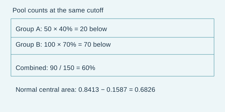
In group A, forty percent of fifty students score below a cutoff. In group B, seventy percent of one hundred students score below the same cutoff. The counts are twenty and seventy. Pooling produces ninety lower scores among one hundred fifty students, giving sixty percent. Averaging forty and seventy produces fifty-five percent and assigns equal influence to groups of unequal size. A two-row table makes the correct weights visible: size, lower-score fraction and lower-score count belong in separate columns.
Ask whether a different comparison is even defined
The pooled calculation works because both groups use the same numerical cutoff and the same definition of below. Two different cutoffs would describe different events, so adding the corresponding counts would not produce the rank of one common score. Similarly, combining a survey of adults with a survey of children may require a carefully stated target population. Arithmetic cannot supply an unstated population definition. In an exam problem, use the described group and resist silently changing what the denominator represents.
Use normal symmetry with a supplied probability
Let a normally distributed variable have mean fifty and standard deviation five. Suppose the question supplies P(X<55)=0.8413. The cutoff forty-five lies equally far below the mean, so symmetry gives P(X<45)=0.1587. The probability between forty-five and fifty-five is 0.8413−0.1587=0.6826. This calculation uses a supplied cumulative value, reflection and subtraction. It does not require memorizing a rounded diagram or treating the height of the density curve as a probability.
Convert a verbal region into an area
A statement such as more than one standard deviation above the mean describes X>55 in this example. Its probability is 1−0.8413=0.1587. More than one standard deviation away from the mean includes both tails and has probability 0.3174. These events differ even though both contain the words one standard deviation. Mark the requested side or sides first, then decide whether you need one tail, two tails, or the central region. For a continuous normal variable, including a single endpoint does not change the probability.
Handle approximations and source limitations explicitly
The selected source captions use coarse percentages when discussing distances from the mean. Such rounded teaching diagrams should not be treated as exact distribution values, and the reported two-standard-deviation percentages are not the usual precise normal probabilities. Our exercises provide the cumulative probability required for the calculation, and the figure labels its areas from that supplied value. A normal assumption also matters: having a mean and a standard deviation does not by itself make a distribution normal or justify normal tail probabilities.
Test transfer with a changed scale
Suppose instead that the mean is eighty and the standard deviation is ten, and the same supplied cumulative probability applies at ninety. The symmetric lower cutoff is seventy. The probability between seventy and ninety remains 0.6826, although the numerical interval is twice as wide as before. What stayed the same was the standardized position, not the raw difference. Finally revisit the pooled groups: if B had only fifty students, the combined rank would become fifty-five percent. The changed population weights explain that different result.
PAUSE & TRYAt a common cutoff, 30 of 50 people in A and 20 of 100 in B are below it. What is the pooled strictly-below percentile?Reveal explanation
100×50/150 = 100/3 percent, about 33.33; add counts before taking the ratio.
Turn the idea into practice.
A fresh set will help you use the relationship with different numbers.
Practice this skillEvidence & editorial note
New statistics source shared by two distinct companions. Selected caption ranges read; original examples and figures; full audiovisual review not performed.
Caption track SHA-256: 2882d532c13cac6889c534c08534285c9af547b1c36cfe6f73d8f9ae683ac372
Source segment references are retained in the catalog. Full captions remain in the local research archive.