
Khan Academy introduces null and alternative hypotheses and relates a p-value to results at least as extreme under a null model. This companion uses a separate exact binomial example and explicitly qualifies the source’s informal normal approximation and causal wording.
Begin with a population claim that could be wrong
A quality team investigates whether a device’s success probability exceeds one half. Let p denote the long-run success proportion for devices produced under the specified process. Before collecting the observations, the team sets a null hypothesis p equals one half and an upper alternative p greater than one half. The parameter refers to a defined process, not just the devices in today’s sample.
For this teaching example, assume eight independent trials with a constant success probability. These assumptions allow an exact binomial model. In a real production study, devices from the same batch might share causes of failure, and the definition of success must be consistent. The mathematical model cannot repair those collection problems after the numbers have been entered.
Specify extreme before looking at the data
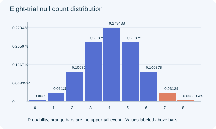
Suppose seven of the eight devices succeed. An upper-tail question treats seven or eight successes as at least as extreme as the observation. It does not count zero or one, because those outcomes point in the opposite direction. It also does not count only exactly seven; results more favorable to the alternative belong in the tail.
The alternative should be specified before observing seven successes. If a team would have switched to a lower-tail question after seeing one success, it has effectively used a different selection rule. That rule needs its own error accounting. Choosing a direction after inspecting the result is not equivalent to the prespecified one-sided test described here.
Compute the conditional tail probability
Under the null probability one half, every sequence of eight binary outcomes has probability one divided by two hundred fifty-six. There are eight sequences with exactly seven successes and one sequence with eight. The upper-tail probability is therefore nine divided by two hundred fifty-six, approximately zero point zero three five two.
The original figure shows the null count distribution and highlights only the seven and eight bars. This p-value assumes the null and the independent-trial model. It asks how often such an extreme statistic would arise under those assumptions. It does not ask how probable the assumptions are after observing the result, and it does not assign a probability to the fixed population parameter.
PAUSE & TRYWould counting only exactly seven successes give the same upper-tail p-value?Reveal explanation
No. It gives 8/256 and omits the more extreme eight-success outcome; the correct tail is 9/256.
Make a decision without replacing uncertainty by proof
If the prespecified significance level is zero point zero five, nine divided by two hundred fifty-six is below that threshold. The team rejects the null and reports evidence that the population success probability exceeds one half, conditional on the model and study conditions. It does not report that every future device succeeds or that the null has been proved impossible.
At a stricter prespecified level of zero point zero one, the same data would not lead to rejection. The evidence has not changed; the decision threshold has. Failing to reject at the stricter level is not proof that the success probability equals one half. Reporting the estimate, the exact p-value and the decision rule lets a reader see these distinct pieces.
Do not confuse a test with a causal experiment
A representative random sample can support a statement about a population success proportion. It cannot by itself identify why the proportion has that value. To claim that a new manufacturing treatment improves success, the investigation needs an appropriate treatment comparison and random assignment, together with careful measurement and relevant scope qualifications.
The source video gives an intuitive hypothesis-testing introduction, but its language near the end is stronger than the statistical argument warrants. A small tail probability is evidence against a specified null model, not a guarantee of a causal drug effect. Our companion separates those issues deliberately: parameter evidence, design validity and causal identification each require their own justification.
Transfer the reasoning to another method carefully
For a mean with unknown population standard deviation, the usual one-sample method uses a t statistic under its conditions. Replacing the unknown spread with a sample estimate does not automatically create an exact normal z test. Large samples can make approximations close, but the procedure should still be named accurately and its assumptions checked.
A final written answer should define the population parameter, state the prespecified hypotheses, justify the model, show the extreme-event calculation and connect the decision to the research question. It should also acknowledge what the study cannot establish. This structure transfers across procedures, while the particular standard error, reference distribution and count checks must change to match the actual statistical method.
Turn the idea into practice.
A fresh set will help you use the relationship with different numbers.
Practice this skillEvidence & editorial note
English captions from 0–685 seconds read. Automatic decimals around 535–581 seconds are ambiguous; no number is copied from that passage. The source uses an estimated SD with a normal approximation; the usual unknown-SD mean procedure is t, not an exact z test. Its final definite-effect language is too strong and its uncontrolled comparison does not independently establish causality. The new exact-probability example below is original. Caption-only review.
Original worked examples, argument and SVGs; short source map only.
Caption track SHA-256: ddfea4385f7a35909c52bffda3acd8d169416117f2650d5bfa19a6b128b7771d
Source segment references are retained in the catalog. Full captions remain in the local research archive.