
StatQuest introduces a bell-shaped distribution and connects its center and width to mean and standard deviation. The companion below develops independent examples and adds explicit cautions about model checking and probability as area.
Begin with the measurement and the group
Before a curve can help, decide what one observation means. Suppose a manufacturer measures the mass of one unopened cereal packet in grams. The observational unit is a packet, the variable is mass, and the target population might be all packets made by one production line during a particular week. Changing any of those definitions changes the question.
A histogram describes the observed sample. A smooth normal curve is a mathematical model used to approximate a population distribution. The two are not identical objects. Even a random sample from a normal population will produce a somewhat uneven histogram. Conversely, a small sample that looks symmetric is not proof that the population follows a normal model.
Separate the center from the spread
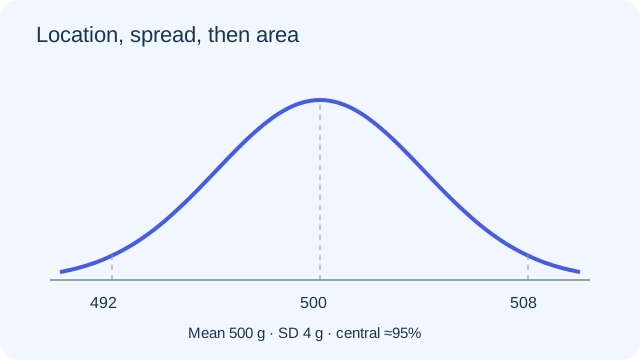
Consider an original example with model mean 500 grams and standard deviation 4 grams. The mean gives the horizontal location of the bell. The standard deviation tells us how far observations typically spread around that location. Neither quantity by itself describes both features.
If the filling process changes so the mean becomes 504 grams while the standard deviation stays 4 grams, the whole model shifts to the right. If the mean stays 500 grams but the standard deviation becomes 8 grams, the distribution spreads out. Its peak becomes lower because the area under a probability-density curve must still total one. A taller peak does not mean the population contains more packets.
Standardize a distance, then interpret it
A packet weighing 508 grams is 8 grams above the mean in the first model. Dividing by the standard deviation gives z = 2. The sign matters: a 492-gram packet has z = −2. These values locate observations relative to a distribution; they are not probabilities.
Standardization also helps compare different measurement scales. A score 10 points above its mean is not automatically more unusual than a score 6 points above another mean. Compare each distance with its own standard deviation. A 10-point difference with SD 20 gives z = 0.5, while a 6-point difference with SD 2 gives z = 3. The second observation is farther from its center in standardized units.
PAUSE & TRYUnder the 500-gram, SD 4-gram model, what is the z-score for 496 grams?Reveal explanation
−1, because (496 − 500)/4 = −1.
Probability is an area across an interval
For a continuous normal variable, the probability of one exact value is zero. This does not mean the measurement is impossible. It means a single point has no width and therefore no area. Real instruments usually report rounded values, so a recorded mass represents a small interval rather than infinite precision.
Under a normal model, approximately 95% of observations lie within two standard deviations of the mean. In the packet example that is the interval from 492 to 508 grams. Approximately 5% lies outside the interval, split equally between the two tails by symmetry. If a question asks for a different boundary, use an appropriate normal-area calculation rather than stretching the empirical rule to an unrelated range.
Check what the model does not promise
The model does not promise that exactly 95 of the next 100 packets fall in the central interval. A probability describes a long-run tendency, and realized counts vary. It also does not justify pooling different production lines if their centers differ; a mixture of populations can have a shape quite unlike one normal distribution.
Look for strong skewness, unusual outliers, truncation and mixtures. Investigate whether measurements were collected consistently and whether a few observations were accidentally duplicated. These checks are part of the statistical argument. They are not decorative steps to add after a calculation has already produced the desired answer.
Write an answer that survives a change of numbers
A strong explanation names the population and variable, states the normal-model assumption, identifies the relevant standardized boundaries, and interprets the resulting area in context. Keep units attached to the original measurements and leave z-scores unitless.
For a self-check, explain why changing grams to kilograms changes the numerical mean and SD but leaves the z-score and interval probability unchanged. Both distances and standard deviation are scaled by the same positive factor. Understanding that cancellation is more durable than memorizing one worked calculation.
Turn the idea into practice.
A fresh set will help you use the relationship with different numbers.
Practice this skillEvidence & editorial note
Real English automatic captions reviewed. The source is a conceptual introduction, not current AP format guidance. Its informal examples of possible normal data do not establish that any particular dataset is normal. Full audiovisual review is pending.
Short source map; original teaching explanation, examples and original SVG diagrams.
Caption track SHA-256: bf7515b3e5cc08778cf27ecb0a76334d155f4cc6890537cc74d51e3199a4bba7
Source segment references are retained in the catalog. Full captions remain in the local research archive.